Use stochastic channels
In this tutorial, we will describe how to use stochastic channels.
In the canonical Hodgkin-Huxley formalism, conductances are deterministic. While each individual channel is stochastic in its opening and closing, there are enough channels that the law of large numbers makes it so that the fluctuations about the mean number of channels open at a given neuronal state (viz. time, membrane potential, intracellular calcium concentration, etc.) is minimal proportional to the mean.
In situations where cells are small, there are few channels, or there is significant thermal noise, it may be useful to model conductances as arising from stochastic ion channels.
Here, we will build a deterministic model and switch to a stochastic model. We will use the Euler-Maruyama method to evolve the system forward in time, using the approximate Langevin method.
Code equivalent to this tutorial can be found in examples/demo_finite_size.m.
Creating the model
We will first create a single-compartment model using Hodgkin-Huxley conductances from Chow et al..
x = xolotl();

x.add('compartment','AB','A',1e-5)

x.AB.add('chow/NaV','gbar',1200);
x.AB.add('chow/Kd','gbar',360);
x.AB.add('Leak','gbar',3,'E',-54.4);
For increased accuracy, we will not approximate channels. This means our simulation will be a little slower, but we will always compute the gating variables by integrating at each time step.
x.approx_channels = 0;
x.stochastic_channels = 1;
We will simulate for 10 seconds.
x.t_end = 10e3;
x.sim_dt = .1;
x.dt = .1;
Setting up the simulation
We ask the question, "How does decreasing the somatic compartment size affect the cell's excitability?" A good way to measure this is to compute the firing rate and interspike interval (ISI) distribution for several cell sizes.
We will sample from to . We will sample 3 times to compute averages.
N = 3;
all_area = logspace(-6, log10(400e-6), 20);
all_f = zeros(length(all_area), N);
Performing the simulations
The simulation is straightforward. We will change the area to the new value, integrate the model, and compute the firing rate from the spike-times.
for j = 1:N
    for i = 1:length(all_area)
        x.reset;
        x.AB.A = all_area(i);
        x.integrate;
        V = x.integrate;
        all_f(i,j) = xtools.findNSpikes(V,0) * x.dt;
    end
end
Visualizing the results
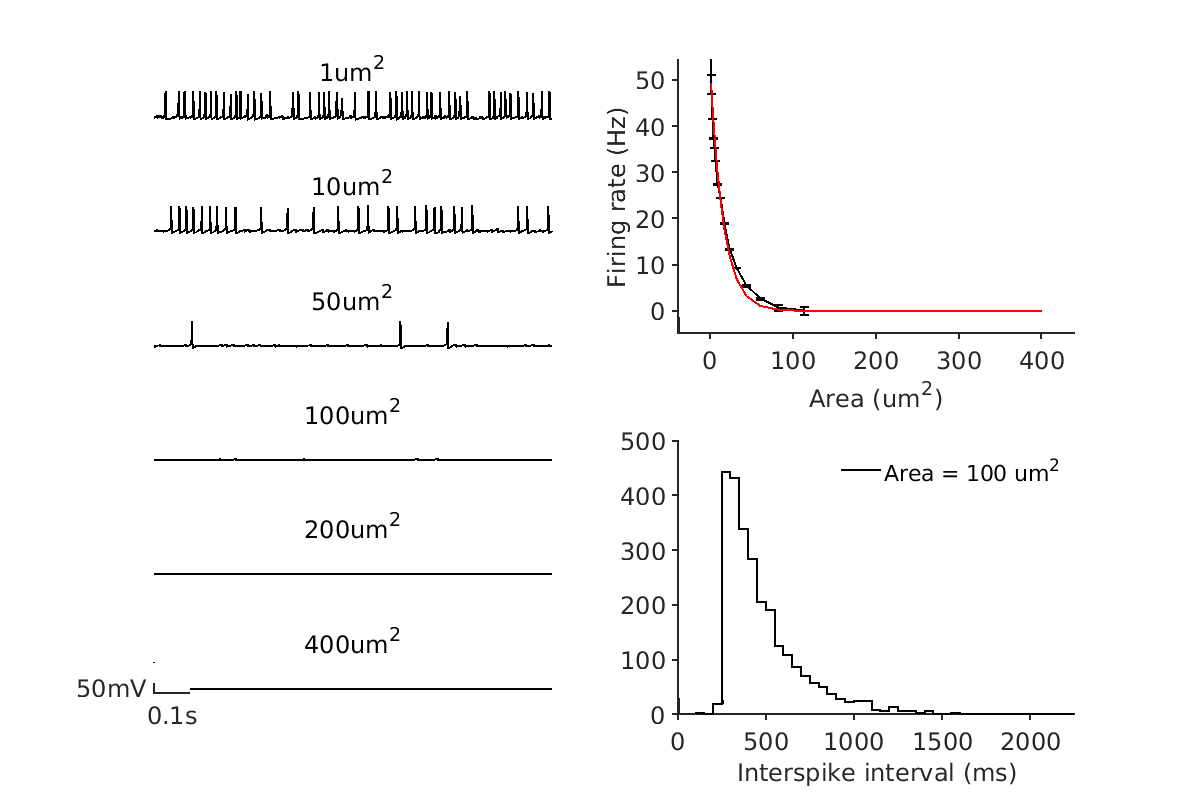
We will plot the voltage traces for selected cell sizes, and also plot the firing rate as a function of cell size. The points will center on the mean of the three trials, and the error bars will be the standard error of the mean. The points seem to follow an exponential, so we will fit one to the data.
Finally, we will plot the ISI distribution as a stair plot for a selected cell size. If the channels were not stochastic, we would expect the cell to reach some sort of steady-state of tonic spiking if sufficiently stimulated.
figure('outerposition',[300 300 1200 901],'PaperUnits','points','PaperSize',[1200 901]); hold on

show_area = [1 10 50 100 200 400]*1e-6;
clear ax
for i = 6:-1:1
    ax(i) = subplot(6,2,(i-1)*2+1); hold on
    x.reset;
    x.AB.A = show_area(i);

    x.integrate;
    V = x.integrate;
    time = (1:length(V))*1e-3*x.dt;
    plot(time,V,'k')
    set(gca,'YLim',[-90 50],'XLim',[0 1])
    th = title([mat2str(x.AB.A*1e6,3) 'um^2']);
    th.FontWeight = 'normal';

    if i < 6
        axis off
    end
end

axf = subplot(2,2,2); hold on
errorbar(all_area*1e6,mean(all_f,2),std(all_f')./mean(all_f,2)','k')
set(gca,'XScale','linear','YScale','linear')
xlabel('Area (um^2)')
ylabel('Firing rate (Hz)')

% fit an exponential
cf = fit(all_area(:),mean(all_f,2),'exp1');
plot(all_area*1e6,cf(all_area),'r')

% also show ISI distribution for 100um^2 neuron
x.reset;
x.AB.A = 10e-6;
x.integrate;
x.t_end = 100e3;
V = x.integrate;
st = xtools.findNSpikeTimes(V,xtools.findNSpikes(V,0));
isis = diff(st);

axisi = subplot(2,2,4); hold on
[hy,hx] = histcounts(isis);
stairs(axisi,hx(2:end)+mean(diff(hx)),hy,'k')
xlabel('Interspike interval (ms)')
legend('Area = 100 um^2')

figlib.pretty('PlotBuffer', 0.1)

axlib.makeEphys(ax(end),'time_scale',.1,'voltage_position',-90)
You should expect to see a plot similar to this (modulo randomness).