Construct models
In this page we will learn how to construct neuron and network models in xolotl from scratch. The first step to constructing any model in xolotl is to create a container for everything we create in it. In this section (and everywhere else), we will use the variable x to hold the xolotl object.
% create a xolotl object
x = xolotl;
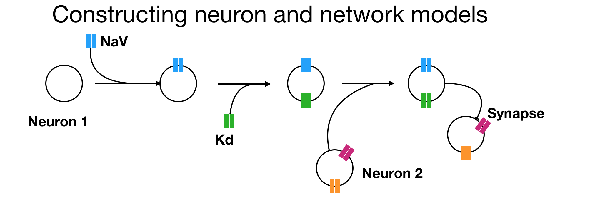
xolotl is a component-oriented simulation environment, which means that all "things" that can exist in the model are pre-defined components; and models are created by linking this components together like building blocks.
xolotl has 4 fundamental types of components:
compartmentObjects of this type are used to represent compartments. Compartments can model entire neurons or parts of neurons. Compartments contain all other component types.conductanceObjects of this type represent populations of ion channels. They are contained within compartments.synapseObjects of this type represent populations of synapses. They connect two different compartments together.mechanismObjects of this type can represent any arbitrary (typically intracellular) mechanism. For example, Calcium buffering is represented as a mechanism.
Create a compartment
The first thing we want to do is create a compartment. A compartment is a piece of neural tissue that shares a common voltage. A compartment can represent a whole neuron, or a small part of one.
To create a compartment, and add it to our xolotl object, we use:
x.add('compartment','AB','A',0.0628)
What we're doing here is creating a compartment and adding it to our xolotl object. This neuron is called AB, and we are specifying that it has a surface area of 0.0628 .
We get a prompt that looks like this:
xolotl object with
---------------------
+ AB
---------------------
This tells us that our xolotl object has one compartment, and its name is AB.
To inspect your xolotl object at any time, simply type its name. Here, since we used a variable called x, we type
x
Add channels to a compartment
OK, let's now add a set of channels to our compartment.
x.AB.add('prinz/NaV','gbar',1000);
x.AB.add('prinz/CaT','gbar',25);
x.AB.add('prinz/CaS','gbar',60);
x.AB.add('prinz/ACurrent','gbar',500);
x.AB.add('prinz/KCa','gbar',50);
x.AB.add('prinz/Kd','gbar',1000);
x.AB.add('prinz/HCurrent','gbar',.1);
Note that, in each line, we are:
- creating a conductance object by specifying the path to the C++ file
- adding it to the compartment "AB"
- Configuring the
gbarparameter in that conductance
The first argument is a character vector that represents a unique path to the C++ header file. For example, if your conductance is specified in
'~/code/xolotl/c++/conductances/prinz/NaV.hpp'
but there are other 'prinz' and 'NaV' conductances, then the character vector
'prinz/NaV' suitably indicates which conductance you mean.
Now, if we look at our model by typing x, we see:
xolotl object with
---------------------
+ AB
  > ACurrent (g=500, E=-80)
  > CaS (g=60, E=30)
  > CaT (g=25, E=30)
  > HCurrent (g=0.1, E=-20)
  > KCa (g=50, E=-80)
  > Kd (g=1000, E=-80)
  > NaV (g=1000, E=50)
---------------------
Add a mechanism
So far, the model consists of a compartment and some channels. There is no mechanism for modeling the influx of Calcium, and its buffering. Let's add a Calcium mechanism:
x.AB.add('prinz/CalciumMech');
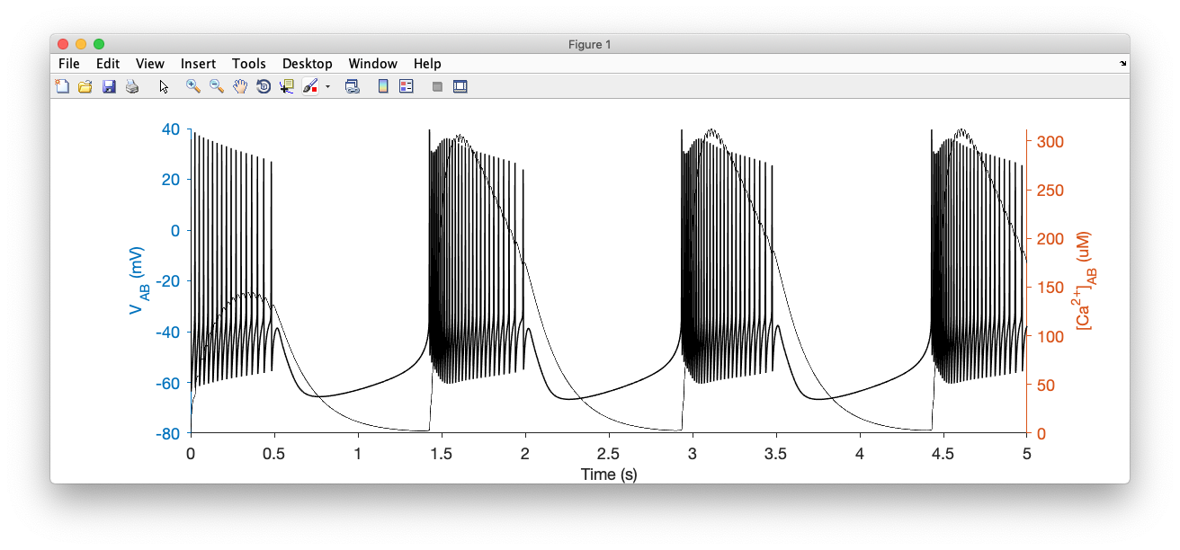
If we integrate and plot the model now, using
x.plot()
we should see something like this:
Wire up compartments using synapses
Let's create another compartment, and connect the two compartments using a synapse
x.add('compartment','LP','A',0.0628)
x.LP.add('prinz/NaV','gbar',1000);
x.LP.add('prinz/Kd','gbar',1000);
Now we can connect the two compartments using a synapse:
x.connect('AB','LP','AlphaSynapse')
Discover parameters and structure of the model
We've just added a new synapse. Let's explore it to understand where it is and what parameters it has. If we look inside the LP compartment using x.LP, we see:
 compartment object (9f24f53) with:

              vol : NaN
                V : -69.0463206551712
              len : NaN
           radius : NaN
               Ca : 0.05
           Ca_out : 3000
       Ca_average : 0.0500000000000942
        Ca_target : NaN
               Cm : 10
         tree_idx : NaN
                A : 0.0628
       neuron_idx : NaN
  shell_thickness : NaN
               Kd : Kd object
              NaV : NaV object
   AlphaSynapseAB : AlphaSynapse object
We see that the AlphaSynapse is included inside the LP neuron. By drilling down into the synapse, we can look at its properties using x.LP.AlphaSynapseAB:
ans =

 AlphaSynapse object (5f2921a) with:

          gmax : 0
      V_thresh : 10
             s : 0
             E : 0
         tau_s : 10
We see that its gmax value, or strength in nS is 0.
Specify initial conditions
Let's set a larger value for the synapse strength. Changing any parameter of the model is as simple as using dot notation:
x.LP.AlphaSynapseAB.gmax = 20;
You can also use the set function.
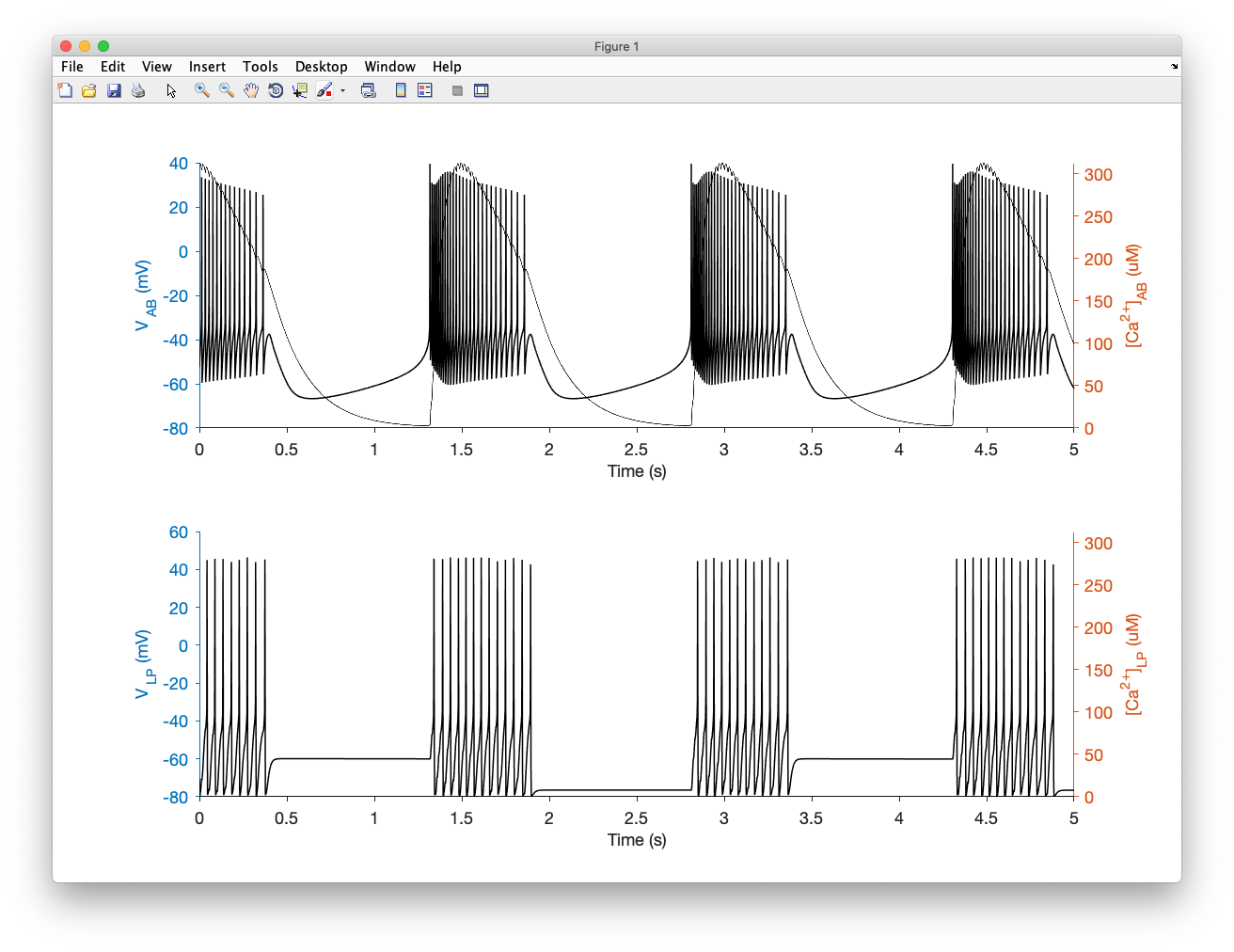
Integrate
We can now integrate and plot the model, and we should see something like this:
How to use this model
We have created a xolotl model with two compartments, several conductances, and synapses connecting the two compartments. If we wanted to perform an experiment where we varied the injected current, or some parameter of the model, we can do so simply by changing the parameters in the object. There is no need to instantiate a new xolotl object for each trial in an experiment. This means that so long as you are using the same model structure (viz. same number of compartments, conductances, connections between them), xolotl doesn't have to recompile. This is super efficient.
If you want to reset your model to where you started, or any other state, you can do so
by creating a snapshot,
and using the reset function.
Warning
Do not create two models with the same structure but different compartment names.
This will confuse xolotl.
If you do so, run xolotl.cleanup.