Fit a model to arbitrary constraints
This document details how to optimize parameters of a xolotl object to fit some constraints using the xfit class.
Parameter optimization is the process of changing some parameters of a model so that the model meets some criteria set by the modeler, as closely as possible. It consists of designing a cost (or objective) function that outputs a positive real-valued result called the cost. The trick is to design a cost function so that when the model does what you want, the cost is very low, and when the model has some aberrant behavior, the cost is very high. We simulate the model and compute the cost for some set of parameters, then algorithmically test new parameters until we find a parameter set that best suits the cost function (by minimizing the cost).
In this document, we will consider a bursting neuron and try to change its maximal conductances to change its burst period to a desired value.
Instantiating the xolotl object
First, let us construct our model. This is an eight-conductance, single-compartment model. Using conductance dynamics from Prinz et al. 2003.
x = xolotl.examples.neurons.BurstingNeuron('prefix', 'prinz');
We will give it some random parameters, by shuffling the existing ones.
x.set('*gbar',veclib.shuffle((x.get('*gbar'))))
This will result in a pathological waveform that probably isn't bursting. Our goal will be to recover bursting activity by algorithmically varying the maximal conductance parameters.
Creating the xfit object
We will create the xfit object, and request the particle swarm algorithm.
This algorithm is a deterministic, black-box optimization scheme.
First, we will make sure that a parallel pool has been created.
This will allow your computer to use more processor cores to perform the optimization faster.
% create a parallel pool using default options
% if one already exists, do nothing
gcp('nocreate');
% create the xfit object
p = xfit('particleswarm');
% tell xfit which xolotl object to use
p.x = x;
% tell xfit to simulate in parallel
p.options.UseParallel = true;
Designing a cost function
We will design a very simple cost function that computes the burst period, the mean number of spikes per burst, and the duty cycle. We aim for a burst period within ms, a mean number of spikes per burst within , and a duty cycle within .
If the model produces a voltage waveform with metrics outside of these values, the returned cost will be large. A model which satisfies this conditions will return a cost of 0.
function C = burstingCostFcn(x,~)

    % x is a xolotl object
    x.reset;
    x.t_end = 10e3;
    x.approx_channels = 1;
    x.sim_dt = .1;
    x.dt = .1;
    x.closed_loop = true;

    % integrate the model and discard the first 10 seconds
    x.integrate;
    % save the second 10 seconds of simulation
    V = x.integrate;

    % measure behavior
    metrics = xtools.V2metrics(V,'sampling_rate',10);

    % accumulate errors
    C = xtools.binCost([950 1050],metrics.burst_period);
    C = C + xtools.binCost([.1 .3],metrics.duty_cycle_mean);
    C = C + xtools.binCost([7 10],metrics.n_spikes_per_burst_mean);

    % safety -- if something goes wrong, return a large cost
    if isnan(C)
        C = 1e3;
    end

end % function
Now, we add the cost function to the xfit object.
p.SimFcn = @xolotl.examples.costfunctions.burstingCostFcn;
Setting up parameter optimization
We will optimize over all maximal conductances.
p.FitParameters = x.find('*gbar')
and we define upper bound and lower bound values for our parameters. These bounds are estimates based on what physiologists know about the expected range of these values.
% lower bound values
p.lb = [100 0 0 0 0 500 0 500];
% upper bound values
p.ub = [1e3 100 100 10 500 2000 0 2000];
Performing the simulation
We display the results before simulation.
% display the results before optimization
figure('outerposition',[300 300 1200 600],'PaperUnits','points','PaperSize',[1200 600]); hold on

subplot(2,1,1); hold on
set(gca,'XLim',[0 10],'YLim',[-80 50])
x.t_end = 10e3;
V = x.integrate;
time = (1:length(V))*1e-3*x.dt;
plot(time,V,'k')
title('Before optimization')

subplot(2,1,2); hold on
set(gca,'XLim',[0 10],'YLim',[-80 50])
and begin the optimization procedure
p.fit;
The results are saved in the seed property of the xfit object,
so we will update our xolotl object with those maximal conductances.
x.set('*gbar', p.seed);
Finally, we can finish our plot, and show voltage waveform produced by the optimized model.
% visualize the results of the optimization
x.t_end = 10e3;
V = x.integrate;
time = (1:length(V))*1e-3*x.dt;
plot(time,V,'r')
title('After optimization')

figlib.pretty('LineWidth', 1, 'PlotLineWidth', 1, 'PlotBuffer', 0)
You should see results that look something like this:
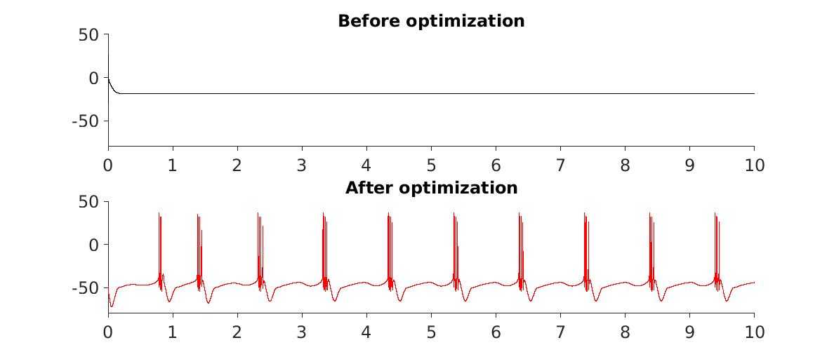
The top trace shows the model before optimization, and the bottom trace shows the results after the optimization algorithm has run its course.
Next steps
We have successfully performed one round of optimization. We could consider performing the optimization multiple times, or varying the initial parameters to try to get a better sense of the parameter space as a whole. It is also possible to run xfit optimizations in a loop to try to find many parameter sets that satisfy the constraints. It is often true in neuronal modeling that many parameter sets, even ones that are very distant from each other, produce similar neuronal activity.