Run simulations in parallel
In this tutorial, we will walk through the process of running multiple simulations in parallel. Doing so can speed up some tasks like parameter sweeps dramatically.
Parallel Computing Toolbox required
You will need the parallel computing toolbox for MATLAB for this tutorial. Make sure you have installed and configured this toolbox correctly, and that you are using as many workers as there threads in your CPU (for most CPUs, the number of threads is equal to twice the number of cores).
Example available
Code in this how-to is available in the script demo_parallel in the examples folder.
Creating the model
We will begin by creating a xolotl model. Here, we will use a bursting neuron model with conductances from Liu et al. 1998. The model is built-in to xolotl as an example, so we will instantiate it.
x = xolotl.examples.neurons.BurstingNeuron('prefix','liu');
x.dt = .1;
x.sim_dt = .1;
x.t_end = 10e3;
We have created an eight-conductance single-compartment model and set the time resolution and total simulation time.
Designing a parameter sweep
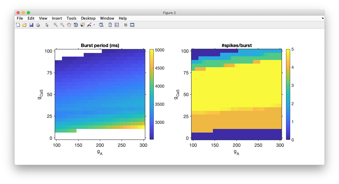
We want to investigate how the slow calcium and A-type potassium currents affect the burst period and number of spikes per burst.
% identify which parameters we want to consider
parameters_to_vary = {'*.CaS.gbar', '*.ACurrent.gbar'};

% create vectors for the parameter values
g_CaS_space = linspace(0,100,25);
g_A_space = linspace(100,300,25);

% create a 2 x N matrix of parameter values
% where N is the number of simulations
% here, N is 25x25 = 625
%
[X, Y] = meshgrid(g_CaS_space, g_A_space);
all_params = [X(:), Y(:)]';
We now have a 2 x N matrix of parameter values corresponding to the cell array of xolotl parameter names, and a matrix containing all combinations of parameter value we want to consider. Since we are varying each parameter through 25 steps, we must perform 625 simulations total.
Creating output vectors
We will store the computed burst periods and mean number of spikes per burst in output vectors.
burst_period = NaN(length(all_params),1);
n_spikes_per_burst = NaN(length(all_params),1);
Running the simulation in parallel
In order to perform the simulation in parallel, we need only use a parfor loop,
which is a parallelized for loop.
Warning
In parfor loops, xolotl properties can be accessed, but not set using object ('dot') notation while in a parfor loop. Instead, use the set method to change parameters.
For each iteration of the loop, we set the xolotl parameters listed in
parameters_to_vary to new values from the all_params matrix.
We then integrate the model to acquire the membrane potential and intracellular calcium traces, cut off a transient region at the beginning of the simulation,
and compute the burst metrics using an xtools function provided in the xolotl distribution.
% first, integrate the model to force it to compile outside the parallel loop
x.integrate;


% run the simulations in parallel
tic
parfor i = 1:length(all_params)
    x.reset;

    x.set('t_end',11e3);
    x.set(parameters_to_vary,all_params(:,i));

    [V,Ca] = x.integrate;


    transient_cutoff = floor(length(V)/2);
    Ca = Ca(transient_cutoff:end,1);
    V = V(transient_cutoff:end,1);

    burst_metrics = xtools.findBurstMetrics(V,Ca);

    burst_period(i) = burst_metrics(1);
    n_spikes_per_burst(i) = burst_metrics(2);


end
t = toc;
Visualizing results
We can make heat-maps of the burst period and mean number of spikes per burst as functions of the varied parameters. A speed of 600X means that we can simulate 600 seconds of data in 1 second. On a 6-core machine from 2013, we achieved speeds greater than 600X.
disp(['Finished in ' mat2str(t,3) ' seconds. Total speed = ' mat2str((length(all_params)*x.t_end*1e-3)/t)])


% assemble the data into a matrix for display
BP_matrix = NaN(length(g_CaS_space),length(g_A_space));
NS_matrix = NaN(length(g_CaS_space),length(g_A_space));
for i = 1:length(all_params)
    xx = find(all_params(1,i) == g_CaS_space);
    y = find(all_params(2,i) == g_A_space);
    BP_matrix(xx,y) = burst_period(i);
    NS_matrix(xx,y) = n_spikes_per_burst(i);
end
BP_matrix(BP_matrix<0) = NaN;
NS_matrix(NS_matrix<0) = 0;

figure('outerposition',[0 0 1200 600],'PaperUnits','points','PaperSize',[1200 600]); hold on

subplot(1,2,1)
imagesc(BP_matrix,'AlphaData',~isnan(BP_matrix));
[L,loc] = axlib.makeTickLabels(g_CaS_space,6);
set(gca,'YTick',loc,'YTickLabels',L)
[L,loc] = axlib.makeTickLabels(g_A_space,6);
set(gca,'XTick',loc,'XTickLabels',L)
ylabel('g_{CaS}')
xlabel('g_A')
title('Burst period (ms)')
axis xy
axis square
colorbar

subplot(1,2,2)
imagesc(NS_matrix,'AlphaData',~isnan(NS_matrix));
[L,loc] = axlib.makeTickLabels(g_CaS_space,6);
set(gca,'YTick',loc,'YTickLabels',L)
[L,loc] = axlib.makeTickLabels(g_A_space,6);
set(gca,'XTick',loc,'XTickLabels',L)
ylabel('g_{CaS}')
xlabel('g_A')
title('#spikes/burst')
axis xy
axis square
colorbar

figlib.pretty();
And you should get something that looks like this: