In this tutorial, we will walk through the process of creating a network model of three neurons connected together by synapses. We will integrate the model to find the membrane potential over time and view the output.

Code equivalent to this tutorial can be found in ../xolotl/examples/demo_stg.m.

A high-level view of the network

Once again, we will approximate a neuron's shape as that of a small spherical object. In our model of the pyloric rhythm of the stomatogastric ganglion of crustaceans, we will consider three model neurons connected with glutamatergic and cholinergic synapses.

Each neuron is understood in this simplification to be a single compartment with a membrane encapsulating ions. Ion channels producing transmembrane conductances lie on the surface of the cell membrane. The intracellular and extracellular concentrations of ions produce the electric potential across the membrane. Synapses connect these neurons together, allowing the membrane potential of one neuron to affect another's.

In xolotl, each neuron is represented by a single compartment object, which contains conductances. Synapses are properties of the xolotl object which connect two compartments together.

First, we set up a generic xolotl object:

x = xolotl;

Making three compartments

Our model of the pyloric rhythm comes from Prinz et al. 2004. The three components of the rhythm are the AB/PD cells, the LP cell, and the PY cells. Since AB and the PDs are strongly electrically coupled, and the PY cells are strongly coupled as well, the model network only consists of three units: an AB/PD, an LP, and a PY. Since we are assuming here that each neuron or composite structure can be adequately represented as a single compartment, we need three compartments.

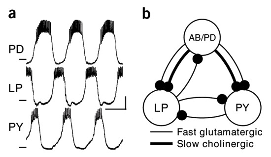
Prinz et al. 2004, Figure 1. (a) shows intracellular voltage recordings in-vitro from three cells in the Jonah crab, Cancer borealis. (b) shows the functional connectivity of the model network, where dots represent post-synaptic targets.

Each compartment will have a surface area of $0.0628~\mathrm{mm^2}$ and a membrane capacitance of $10~\mathrm{nF}$.

% create three compartments named AB, LP, and PY
x.add('compartment', 'AB', 'Cm', 10, 'A', 0.0628);
x.add('compartment', 'LP', 'Cm', 10, 'A', 0.0628);
x.add('compartment', 'PY', 'Cm', 10, 'A', 0.0628);

If you inspect the xolotl object in the command window, you should see something like this:

>> x

xolotl object with
---------------------
+ AB  
---------------------
+ LP  
---------------------
+ PY  
---------------------

We have now constructed our three compartments (with nothing in them).

Adding conductances

Each compartment in our model will have eight conductances:

• NaV, a fast, inactivating sodium conductance;
• CaT, a transient calcium conductance;
• CaS, a slow calcium conductance;
• ACurrent, an A-type potassium conductance;
• KCa, a calcium-gated potassium conductance;
• Kd, a delayed rectifier potassium conductance;
• HCurrent, a hyperpolarization-activated rectifying conductance; and
• Leak, the passive leak current.

In xolotl, these conductances are defined within the ../c++/conductances/prinz/ folder. We can add them each one by on, or we can get fancy. Let's get fancy.

The conductances we want are:

conds = {'NaV', 'CaT', 'CaS', 'ACurrent', 'KCa', 'Kd', 'HCurrent', 'Leak'};

And, looking at the paper, the maximal conductances (in $\mathrm{\mu S / mm^2}$) are:

% for AB/PD
gbars(:, 1) = [1000, 25, 60, 500, 50, 1000, 0.1,   0];
% for LP
gbars(:, 2) = [1000,  0, 40, 200,  0,  250, 0.5, 0.3];
% for PY
gbars(:, 3) = [1000, 24, 20, 500,  0, 1250, 0.5, 0.1];

The reversal potentials are determined by the ionic species fluxed by each conductance and are the same for each compartment.

reversal =         [50, 30, 30, -80, -80, -80, -20, -50];

Adding all conductances to the compartments:

comps       = x.find('compartment');
% for each compartment
for ii = 1:length(comps)
    % for each Prinz conductance
    for qq = 1:length(conds)-1
    % add the conductance to the compartment
        x.(comps{ii}).add(['prinz/' conds{qq}], 'gbar', gbars(qq, ii), 'E', reversal(qq));
    end
    % add the Leak conductance
    x.(comps{ii}).add(conds{end}, 'gbar', gbars(end, ii), 'E', reversal(end));
end

We used two loops to add all the conductances to the compartments. For example, the ii=1, qq=1 case is equivalent to:

x.AB.add('prinz/NaV', 'gbar', 1000, 'E', 50);

The xolotl object should look like this:

>> x

xolotl object with
---------------------
+ AB  
  > ACurrent (g=500, E=-80)
  > CaS (g=60, E=30)
  > CaT (g=25, E=30)
  > HCurrent (g=0.1, E=-20)
  > KCa (g=50, E=-80)
  > Kd (g=1000, E=-80)
  > Leak (g=0, E=-50)
  > NaV (g=1000, E=50)
---------------------
+ LP  
  > ACurrent (g=200, E=-80)
  > CaS (g=40, E=30)
  > CaT (g=0, E=30)
  > HCurrent (g=0.5, E=-20)
  > KCa (g=0, E=-80)
  > Kd (g=250, E=-80)
  > Leak (g=0.3, E=-50)
  > NaV (g=1000, E=50)
---------------------
+ PY  
  > ACurrent (g=500, E=-80)
  > CaS (g=20, E=30)
  > CaT (g=24, E=30)
  > HCurrent (g=0.5, E=-20)
  > KCa (g=0, E=-80)
  > Kd (g=1250, E=-80)
  > Leak (g=0.1, E=-50)
  > NaV (g=1000, E=50)
---------------------

All conductances have been successfully added!

Other ways we could have done this: the cpplab.search('conductances/prinz/') method would have given us a list of all the conductances from Prinz et al. 2004. In the paper, the conductances aren't in alphabetical order, here they would be. It's up to preference.

Adding calcium dynamics

Since some of these conductances (CaT, CaS, and KCa) depend on the intracellular calcium concentration, we also need a calcium mechanism CalciumMech1 for each compartment.

for ii = 1:length(comps)
    x.(comps{ii}).add('CalciumMech1');
end

Adding synapses

Synapses connect our compartments together. In the stomatogastric circuit, there are two inhibitory synapse types, one that is glutamatergic, and one that is cholinergic. We can use the connect function to create synapses. For example,

x.connect('AB', 'LP', 'prinz/Cholinergic', 'gbar', 30);

creates a cholinergic synapse from AB to LP with a specified maximal conductance of $30~\mathrm{\mu S}$.

Add all the synapses:

x.connect('AB','LP','prinz/Chol','gbar',30);
x.connect('AB','PY','prinz/Chol','gbar',3);
x.connect('AB','LP','prinz/Glut','gbar',30);
x.connect('AB','PY','prinz/Glut','gbar',10);
x.connect('LP','PY','prinz/Glut','gbar',1);
x.connect('PY','LP','prinz/Glut','gbar',30);
x.connect('LP','AB','prinz/Glut','gbar',30);

You can inspect synapses by viewing x.synapses which is a vector of cpplab objects.

Simulating the model

Let's simulate the model for 5 seconds.

x.t_end = 5000;

We can now integrate the model to compute the voltage, ionic and synaptic currents.

[V, ~, ~, currs, syns] = x.integrate;

Plot the membrane potential

C = x.find('compartment');
figure('outerposition',[100 100 1000 900],'PaperUnits','points','PaperSize',[1000 900]);
hold on
for i = 1:3
    subplot(3,1,i); hold on
    plot(V(:,i))
    ylabel('V_m (mV)')
    title(C{i})
end

Plot the ionic currents

figure('outerposition',[100 100 1000 900],'PaperUnits','points','PaperSize',[1000 900]);
hold on
subplot(3,1,1); hold on
plot(currs(:,1:7))
ylabel('I (nA)')
title(C{1})
legend(x.(C{1}).find('conductance'))

subplot(3,1,2); hold on
plot(currs(:,8:15))
title(C{2})
ylabel('I (nA)')
legend(x.(C{2}).find('conductance'))

subplot(3,1,3); hold on
plot(currs(:,16:23))
title(C{3})
ylabel('I (nA)')
legend(x.(C{3}).find('conductance'))

Plot the synaptic currents

figure('outerposition',[100 100 1000 500],'PaperUnits','points','PaperSize',[1000 500]);
hold on

plot(syns)
ylabel('I (nA)')
title('synaptic currents')