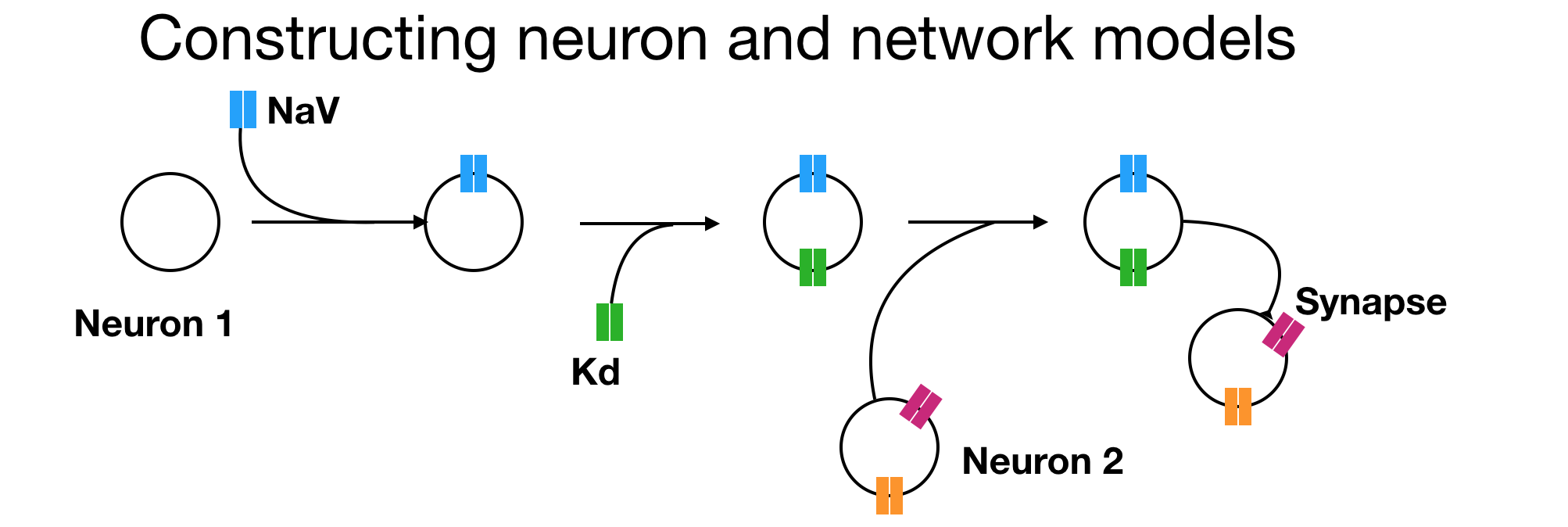
In this page we will learn how to construct neuron and network models in xolotl from scratch. The first step to constructing any model in xolotl is to create a container for everything we create in it. In this section (and anywhere else), we will use the variable x to hold the xolotl object.
% create a xolotl object
x = xolotl;
xolotl is a component-oriented simulation environment, which means that all "things" that can exist in the model are pre-defined components; and models are created by linking this components together like building blocks.
xolotl has 4 fundamental types of components:
compartmentObjects of this type are used to represent compartments. Compartments can model entire neurons or parts of neurons. Compartments contain all other component types.conductanceObjects of this type represent populations of ion channels. They are contained within compartments.synapseObjects of this type represent populations of synapses. They connect two different compartments together.mechanismObjects of this type can represent any arbitrary (typically intracellular) mechanism. For example, Calcium buffering is represented as a mechanism.
The first thing we want to do is create a compartment. A compartment is a piece of neural tissue that shares a common voltage. A compartment can represent a whole neuron, or a small part of one.
To create a compartment, we use:
x.add('compartment','exampleNeuron','A',.01)
What we're doing here is creating a compartment and adding it to our xolotl object. This neuron is called exampleNeuron, and we are specifying that it has a surface area of 0.1 mm^2.
We get a prompt that looks like this:
xolotl object with
---------------------
+ exampleNeuron
---------------------
This tells us that our xolotl object has one compartment, and its name is exampleNeuron.
To inspect your xolotl object at any time, simply type its name. Here, since we used a variable called x, we type
x
Compartments
Compartments represent three-dimensional sections of membrane. A neuron can consist of one or more compartments. In multi-compartment neurons, axial synapses with very fast kinetics connect compartments. Compartments in different neurons can be connected with chemical or electrical synapses.
You can create a compartment (independent of a xolotl object) using cpplab.
% create a compartment with a specified volume
AB = cpplab('compartment', 'vol', 0.01)
AB is a free-floating object. You can inspect it like you would any other MATLAB object.
>>  AB

AB =

compartment object with:

     hash : 44c3772
       Cm : 10
        A : 0.01
   radius : NaN
      vol : NaN
  Ca_average : NaN
  shell_thickness : NaN
  tree_idx : NaN
        V : -60
  neuron_idx : NaN
  Ca_target : NaN
       Ca : NaN
   Ca_out : 3000
      len : NaN
You can add it to your xolotl object.
% add compartment AB to the xolotl object tree
x.add('AB', AB)
A handy shortcut for this is
% add a compartment named AB with a specified volume
x.add('compartment', 'AB', 'vol', 0.01)
We will use this shortcut extensively in the documentation, but remember that you can always do things the "long" way.
There are many useful properties of each compartment object:
The hash is an alphanumeric MD5 hash unique to the structure of this compartment.
The specific membrane capacitance is Cm in .
* The membrane potential is V in .
Size and shape of compartments
Compartments are assumed to be specified by their size or shape. In the case of size, compartments have a defined surface area A (). If shape is instead defined, the compartment is assumed to be cylindrical with a radius and len (length). The surface area is then computed to be in single-compartment cases (and potentially lacking the cylindrical surface areas in the case of multi-compartment models). If the radius and length are defined (which they must be in multi-compartment cases), then the A property is ignored. Similarly, the compartment volume is contained within the vol property. In the case of a cylindrical compartment with defined radius and length, the volume is defined to be .
Calcium properties
Cacontains the intracellular calcium concentration in M.Ca_outcontains the extracellular calcium concentration in M.- Calcium is buffered very rapidly upon passing through the cell membrane. Many models compute intracellular calcium concentration with respect to the volume of an interior "shell." This value is stored in
shell_thicknessin mm. - In homeostatic tuning models, it is sometimes important to keep track of an average intracellular calcium concentration,
Ca_averagein M. - In homeostatic tuning models, it is sometimes important to keep track of a target intracellular calcium concentration,
Ca_targetin M.
Conductances
A conductance object can be created using cpplab.
% instantiate the fast sodium conductance from Prinz et al. 2003
>> NaV = cpplab('prinz/NaV', 'gbar', 1000, 'E', 50)
NaV =

 NaV object with:

          hash : a85ae87
          gbar : 1000
             E : 50
             m : NaN
             h : NaN
There are a few useful properties in each conductance object:
The MD5 hash of this object.
gbar contains the specific maximal conductance in .
E contains the reversal potential in .
m contains the activation gating variable (unitless).
* h contains the (de)inactivation gating variable (unitless).
What conductances are available?
All C++ header files which define the conductances used in xolotl are contained in the c++/conductances folder in the xolotl directory. If you are unsure where this is, type this into your MATLAB prompt:
fileparts(fileparts(which('xolotl')))
You can also list all conductances with
cpplab.search('conductances')
Synapses
Synapses connect compartments together. Synapses are stored in a vector of cpplab objects. Synapse objects contain the following properties:
- The MD5
hashof this object. gbarcontains the maximal conductance in .scontains the synaptic gating variable (unitless).
Synapses are created between two compartments using the connect function:
% connect compartments AB and PD with an electrical synapse
x.connect('AB', 'PD')
% connect two compartments with an electrical synapse
% and specify properties
x.connect('AB', 'PD', 'gbar', 100)
% connect two compartments with a glutamatergic synapse
% kinetics from Prinz et al. 2004
x.connect('AB', 'LP', 'prinz/Glut')
% connect two compartments with a glutamatergic synapse
% and specify properties
x.connect('AB', 'LP', 'prinz/Glut', 'gbar', 100)
What synapses are available?
All C++ header files which define the synapses used in xolotl are contained in the c++/synapses folder in the xolotl directory. If you are unsure where this is, type this into your MATLAB prompt:
fileparts(fileparts(which('xolotl')))
You can also list all synapses with
cpplab.search('synapses')
Mechanisms
The add function and the object tree
The general-purpose add function adds cpplab objects to the xolotl tree. In brief, a cpplab object is a special type of MATLAB data structure that secretly binds MATLAB code to C++ code. The advantage of this is that the user gets to work entirely in MATLAB but simulations run with the full power and speed of C++.
xolotl itself is a framework for creating and integrating neuronal and network models using cpplab.
What can be added to what?
compartments are added directly to the xolotl object. conductances are added to compartments. synapses connect two compartments together but themselves are properties of the xolotl object. mechanisms are special types of cpplab objects that affect how xolotl performs computations. They include stochastic noise, calcium integration, homeostatic tuning, and so on. As such, they can be added to compartments or conductances.
Exploring constructed models in the command line
xolotl objects are bona fide MATLAB objects and can be readily manipulated in the command line.
Here is an example of a xolotl object, representing the structure of a stomatogastric ganglion model from crustacea published in Prinz et al. 2004. The code to produce this model can be found in examples/demo_stg.m.
>> x

xolotl object with
---------------------
+ AB
  > ACurrent (g=500, E=-80)
  > CaS (g=60, E=26.173778091544)
  > CaT (g=25, E=26.173778091544)
  > HCurrent (g=0.1, E=-20)
  > KCa (g=50, E=-80)
  > Kd (g=1000, E=-80)
  > NaV (g=1000, E=50)
---------------------
+ LP
  > ACurrent (g=200, E=-80)
  > CaS (g=40, E=76.6764125879106)
  > CaT (g=0, E=76.6764125879106)
  > HCurrent (g=0.5, E=-20)
  > KCa (g=0, E=-80)
  > Kd (g=250, E=-80)
  > Leak (g=0.3, E=-50)
  > NaV (g=1000, E=50)
---------------------
+ PY
  > ACurrent (g=500, E=-80)
  > CaS (g=20, E=62.3932795257928)
  > CaT (g=24, E=62.3932795257928)
  > HCurrent (g=0.5, E=-20)
  > KCa (g=0, E=-80)
  > Kd (g=1250, E=-80)
  > Leak (g=0.1, E=-50)
  > NaV (g=1000, E=50)
---------------------
Displaying the xolotl object shows select properties of each conductance within each compartment. We can see that there are three compartments each with 7-8 conductances with varied maximal conductances. In addition, we can infer that the sodium channels have reversal potentials of and the potassium channels of .
In MATLAB, all compartments and conductances in this view are hyperlinked and can be clicked on to view that particular object. We can also access this view through the command line. Let's look at the first compartment.
>> x.AB

ans =

 compartment object with:

             hash : bba3847
               Cm : 10
                A : 0.0628
  shell_thickness : NaN
         tree_idx : NaN
              vol : NaN
                V : -48.7425773412141
        Ca_target : NaN
       Ca_average : 97.5752632857105
       neuron_idx : NaN
              len : NaN
           radius : NaN
               Ca : 354.000031181001
           Ca_out : 3000
              NaV : NaV object
         HCurrent : HCurrent object
     CalciumMech1 : CalciumMech1 object
              CaS : CaS object
              KCa : KCa object
         ACurrent : ACurrent object
               Kd : Kd object
              CaT : CaT object
We see all the properties of a standard compartment object plus each of the conductances added to the xolotl tree (using the add function). We can look closer at a conductance.
>> x.AB.NaV

ans =

 NaV object with:

          hash : a85ae87
          gbar : 1000
             m : 0.0107532302761698
             h : 0.64304369213413
             E : 50
Since these are MATLAB objects, we can edit the properties in-situ.
% set AB's NaV maximal conductance to zero
>> x.AB.NaV.gbar = 0

xolotl object with
---------------------
+ AB
  > ACurrent (g=500, E=-80)
  > CaS (g=60, E=26.173778091544)
  > CaT (g=25, E=26.173778091544)
  > HCurrent (g=0.1, E=-20)
  > KCa (g=50, E=-80)
  > Kd (g=1000, E=-80)
  > NaV (g=0, E=50)
---------------------
+ LP
  > ACurrent (g=200, E=-80)
  > CaS (g=40, E=76.6764125879106)
  > CaT (g=0, E=76.6764125879106)
  > HCurrent (g=0.5, E=-20)
  > KCa (g=0, E=-80)
  > Kd (g=250, E=-80)
  > Leak (g=0.3, E=-50)
  > NaV (g=1000, E=50)
---------------------
+ PY
  > ACurrent (g=500, E=-80)
  > CaS (g=20, E=62.3932795257928)
  > CaT (g=24, E=62.3932795257928)
  > HCurrent (g=0.5, E=-20)
  > KCa (g=0, E=-80)
  > Kd (g=1250, E=-80)
  > Leak (g=0.1, E=-50)
  > NaV (g=1000, E=50)
---------------------
Hashing a model
Each xolotl object is hashed by the MD5 algorithm to determine a unit alphanumeric identifier. Two xolotl objects are different only if their underlying structure (compartments, types of conductances, synapses) are different -- not if parameters are different.
% hash a xolotl object
>> x

xolotl object with
---------------------
+ AB
  > ACurrent (g=5, E=-80)
  > CaS (g=0.113, E=30)
  > CaT (g=0.191, E=30)
  > HCurrent (g=0.128, E=-20)
  > KCa (g=0.163, E=-80)
  > Kd (g=0.11, E=-80)
  > Leak (g=0.099, E=-50)
  > NaV (g=0.181, E=30)
---------------------
>> x.hash

ans =

    '6b3a55344dbd63074cfd703061f9ae4d'
>> % the hash doesn't change when you change the parameters

>> x.AB.ACurrent.gbar = 0;

>> x.hash

ans =
    '6b3a55344dbd63074cfd703061f9ae4d'
Multi-compartment models
Geometry
The Axial synapse
The slice method
Visualization
Using the built-in plot function
Manipulating models
Writing custom plot functions that can be manipulated
Creating new conductances
Understanding the conductance class
Manually
Using the conductance class
Where should I put them?
All conductances (and any other network component) are defined by
an .hpp header file and live in the xolotl directory under xolotl/c++/conductances/.
Within that directory, conductances are grouped by the surname of the first
author on the paper from where they were sourced. For example, conductances
from Liu et al. 1998 can be found in xolotl/c++/conductances/liu/.
If an author, such as Farzan Nadim or Cristina Soto-Trevino happens to have
papers over multiple years, the last two digits of the paper publishing year
are appended to the author name (e.g. ../nadim98). If there are multiple
papers in a single year, lowercase alphabetical indices are used (e.g. ../golowasch01a).
If a paper, such as Soplata et al. 2017 describes multiple channels of a
single type in different cell types (e.g. thalamocortical relay and thalamic
reticular cells), then full-word descriptions can be used, such as
(../soplata/thalamocortical).
Creating new synapses
Understanding the synapse class
Creating new mechanisms
Understanding the mechanism class
Diving deeper: cpplab
Troubleshooting
Controlling Verbosity
x.verbosity = 99;
Need a table to tell the user what each value of verbosity does.
Resetting the cpplab path cache
You can rebuild the cache with:
cpplab.rebuildCache()
If that doesn't work, you can forcibly delete the cache with:
delete(which('paths.cpplab'))